Plot size

Mar 4, 2026

Updated: Mar 20, 2026

voidxno

An attempt to quantify real-life MMX plot size patterns into charts, tables and formulas. Created by plotting lots of different k-sizes and C-levels. Both to find patterns, and make sure of them. Goal is an easy overview of plot size behavior, with solid numbers as a bonus.

TLDR;

• Compression resistant plot format
• Given a specific k-size/C-level, following is true:
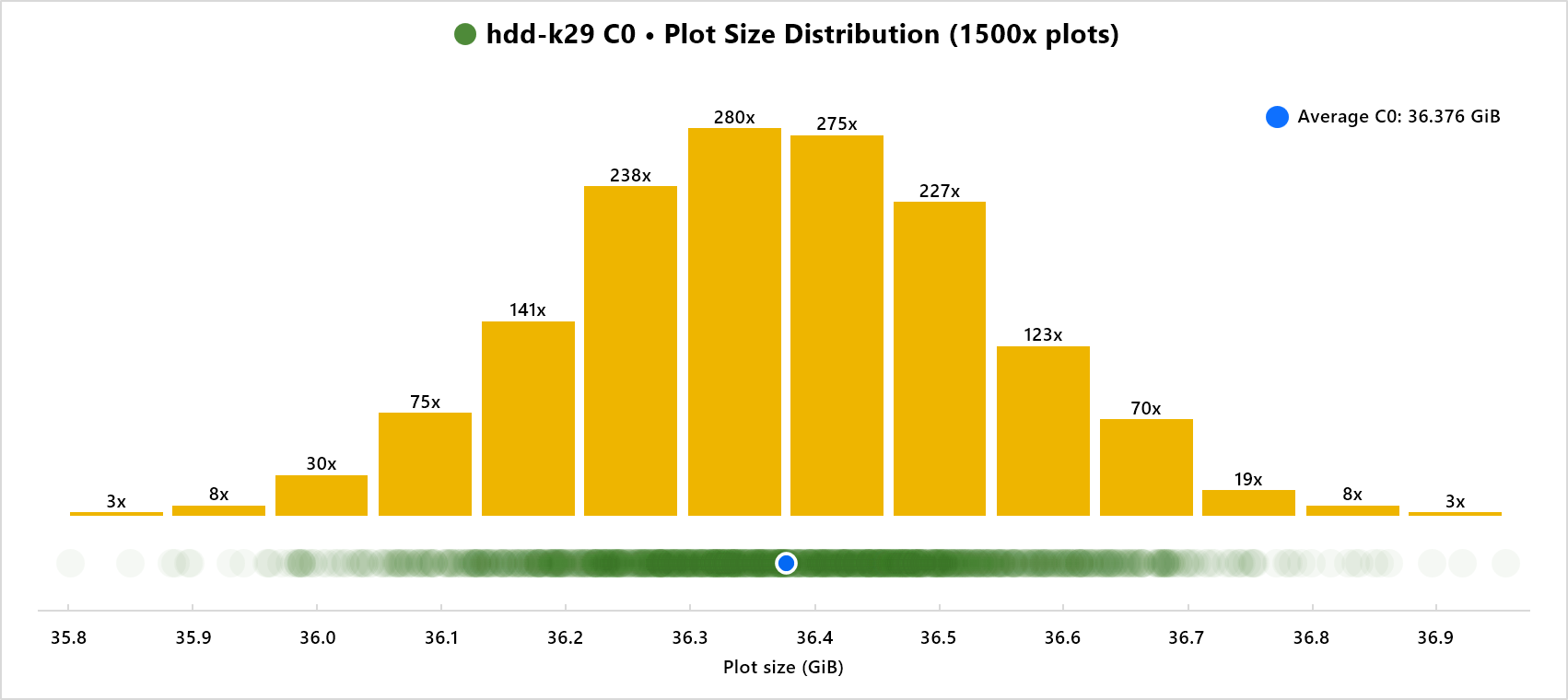
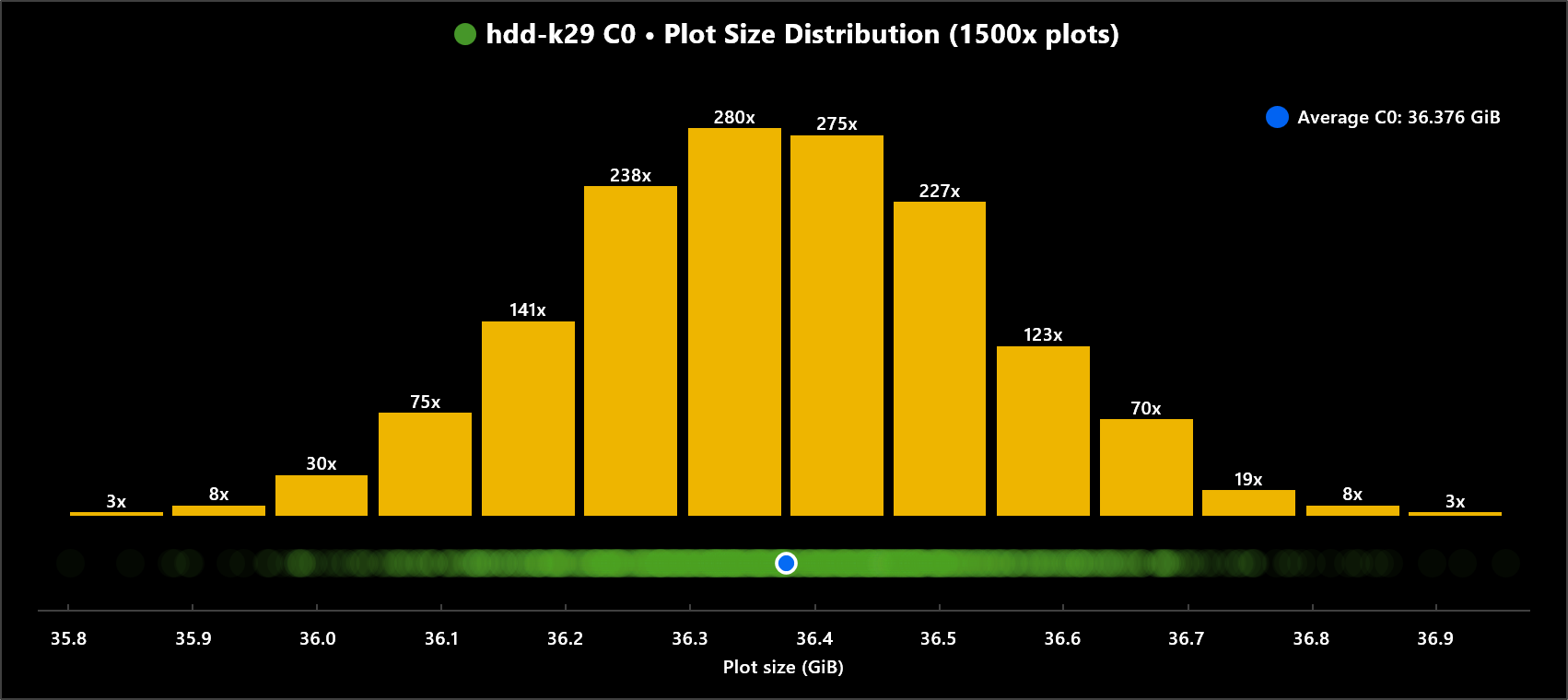
  • Plot size is random, within a small bell curved range
  • Plot size will average out, given enough plots
  • Varying size equals less or more proofs, not better compression
• Given specific k-size, following is true:
  • Delta size between C-levels is identical, linear
  • Delta size of distribution bell curve is identical for all C-levels
• Evaluate yourself what C-compression level is worth it
• A few thoughts about filling a disk further down
• Own section below with data for SSD-plots

Charts

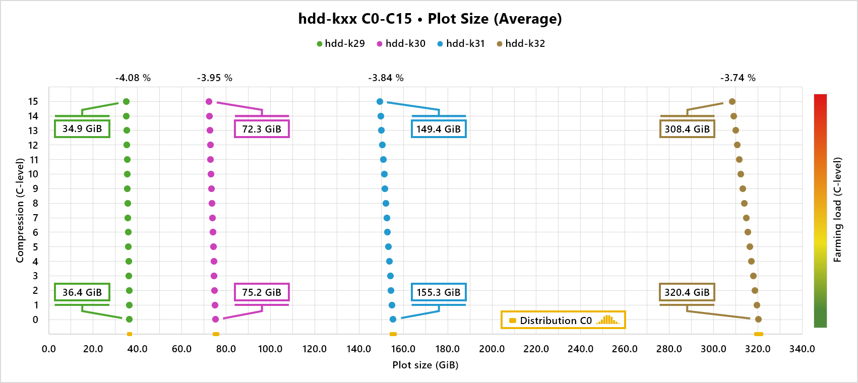
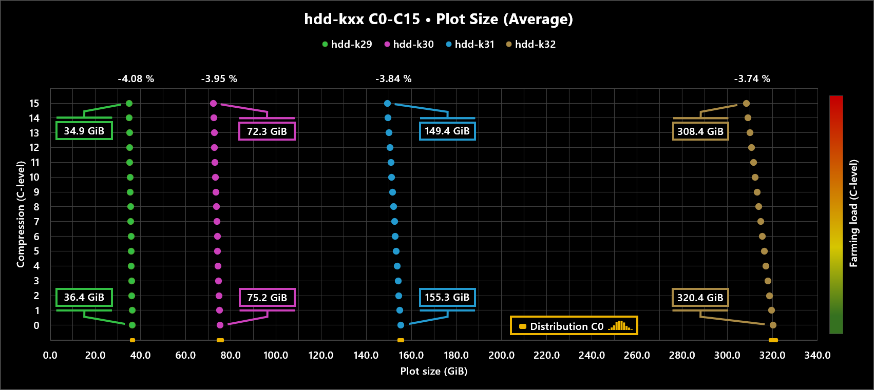
First chart is an overall overview using formulas created. Followed by two charts using real-life hdd-k29 plotting data to illustrate patterns. Those patterns repeat in other k-sizes. Decimal GiB numbers in overview chart have been rounded up. Less chance of underestimating combined size of plots.

Overview

Distribution (hdd-k29, C0)

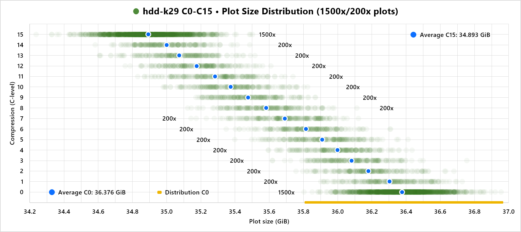
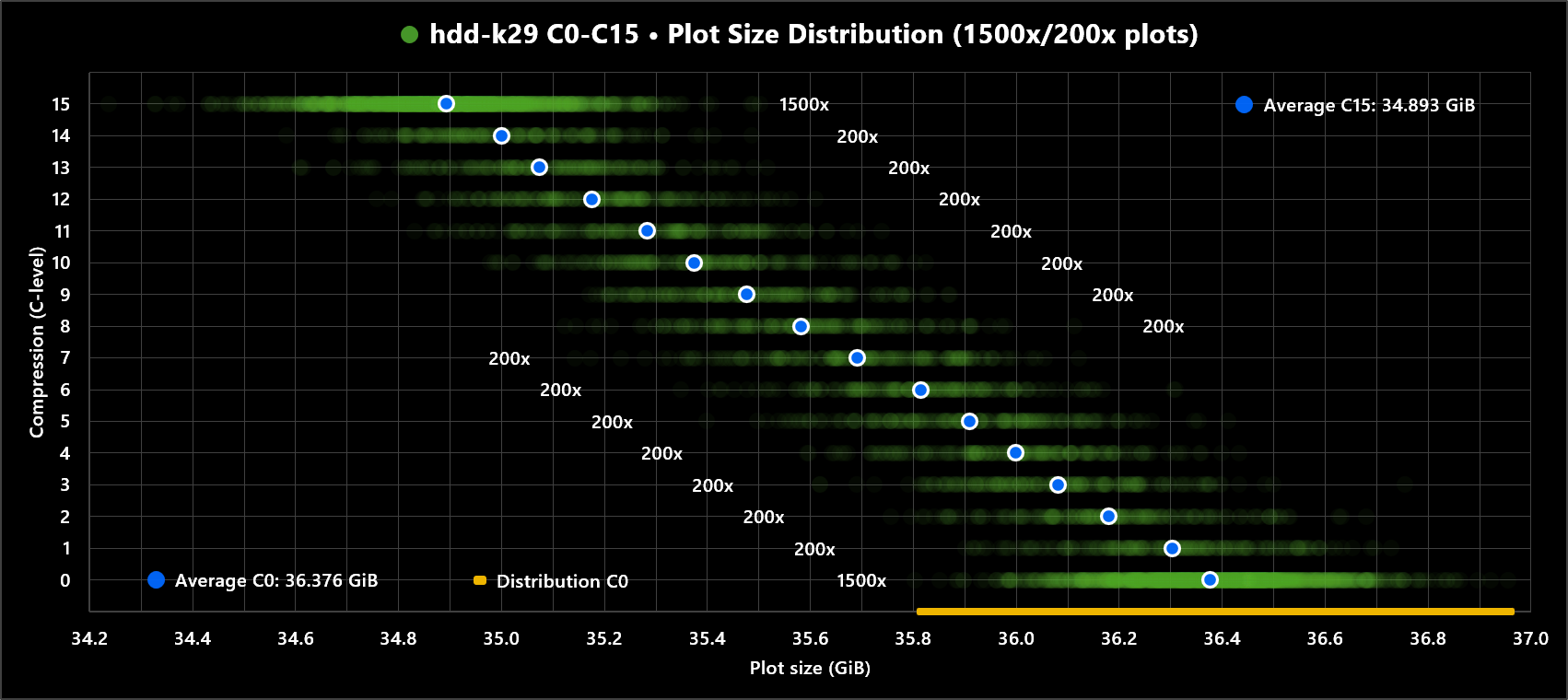
Distribution (hdd-k29, C0-C15)

Average

List

	hdd-k29	hdd-k30	hdd-k31	hdd-k32
C0	36.376 GiB	75.196 GiB	155.279 GiB	320.321 GiB
C15	34.893 GiB	72.223 GiB	149.315 GiB	308.351 GiB
%	-4.08 %	-3.95 %	-3.84 %	-3.74 %

Full list

	hdd-k29	hdd-k30	hdd-k31	hdd-k32
C0	36.376 GiB	75.196 GiB	155.279 GiB	320.321 GiB
C1	36.277 GiB	74.998 GiB	154.882 GiB	319.523 GiB
C2	36.178 GiB	74.800 GiB	154.484 GiB	318.725 GiB
C3	36.079 GiB	74.602 GiB	154.086 GiB	317.927 GiB
C4	35.980 GiB	74.404 GiB	153.689 GiB	317.129 GiB
C5	35.882 GiB	74.205 GiB	153.291 GiB	316.331 GiB
C6	35.783 GiB	74.007 GiB	152.894 GiB	315.533 GiB
C7	35.684 GiB	73.809 GiB	152.496 GiB	314.735 GiB
C8	35.585 GiB	73.611 GiB	152.098 GiB	313.937 GiB
C9	35.486 GiB	73.412 GiB	151.701 GiB	313.139 GiB
C10	35.387 GiB	73.214 GiB	151.303 GiB	312.341 GiB
C11	35.288 GiB	73.016 GiB	150.905 GiB	311.543 GiB
C12	35.189 GiB	72.818 GiB	150.508 GiB	310.745 GiB
C13	35.091 GiB	72.620 GiB	150.110 GiB	309.947 GiB
C14	34.992 GiB	72.421 GiB	149.713 GiB	309.149 GiB
C15	34.893 GiB	72.223 GiB	149.315 GiB	308.351 GiB
%	-4.08 %	-3.95 %	-3.84 %	-3.74 %

Formula

• HDD-plot C0 (GiB): 4.98452*k*1.99844^(k-30.99297)+0.00513
• HDD-plot C15 (%): -(1.0871^(34.1291-k)+2.5423)

Distribution

Nearly all plots will be within a 99.5% GiB range, with average plot size in middle. Given enough plots there will be a few outliers, but not many. 99.5% is a representative value for a practical range. GiB numbers with one decimal place have been rounded up and down to best fit purpose. Less chance of underestimating average plot sizes and range values.

List

	hdd-k29	hdd-k30	hdd-k31	hdd-k32
99.5%	±0.485 GiB	±0.729 GiB	±1.082 GiB	±1.586 GiB
C0 (average)	36.4 GiB	75.2 GiB	155.3 GiB	320.4 GiB
C0 (range)	35.8 - 36.9	74.4 - 76.0	154.1 - 156.4	318.7 - 322.0

Full list

	hdd-k29	hdd-k30	hdd-k31	hdd-k32
25%	±0.052 GiB	±0.078 GiB	±0.116 GiB	±0.170 GiB
50%	±0.113 GiB	±0.169 GiB	±0.251 GiB	±0.369 GiB
75%	±0.195 GiB	±0.293 GiB	±0.435 GiB	±0.638 GiB
99.5%	±0.485 GiB	±0.729 GiB	±1.082 GiB	±1.586 GiB
C0	35.8 - 36.9	74.4 - 76.0	154.1 - 156.4	318.7 - 322.0
C1	35.7 - 36.8	74.2 - 75.8	153.7 - 156.0	317.9 - 321.2
C2	35.6 - 36.7	74.0 - 75.6	153.4 - 155.6	317.1 - 320.4
C3	35.5 - 36.6	73.8 - 75.4	153.0 - 155.2	316.3 - 319.6
C4	35.4 - 36.5	73.6 - 75.2	152.6 - 154.8	315.5 - 318.8
C5	35.3 - 36.4	73.4 - 75.0	152.2 - 154.4	314.7 - 318.0
C6	35.2 - 36.3	73.2 - 74.8	151.8 - 154.0	313.9 - 317.2
C7	35.1 - 36.2	73.0 - 74.6	151.4 - 153.6	313.1 - 316.4
C8	35.1 - 36.1	72.8 - 74.4	151.0 - 153.2	312.3 - 315.6
C9	35.0 - 36.0	72.6 - 74.2	150.6 - 152.8	311.5 - 314.8
C10	34.9 - 35.9	72.4 - 74.0	150.2 - 152.4	310.7 - 314.0
C11	34.8 - 35.8	72.2 - 73.8	149.8 - 152.0	309.9 - 313.2
C12	34.7 - 35.7	72.0 - 73.6	149.4 - 151.6	309.1 - 312.4
C13	34.6 - 35.6	71.8 - 73.4	149.0 - 151.2	308.3 - 311.6
C14	34.5 - 35.5	71.6 - 73.2	148.6 - 150.8	307.5 - 310.8
C15	34.4 - 35.4	71.4 - 73.0	148.2 - 150.4	306.7 - 310.0

Formula

• HDD-plot k29 (±GiB): 0.153*sinh(0.00872*p)-0.0632*ln(100-p)+0.2911
• HDD-plot k-size (multiplier): 2.386E-18*k^12.05

Filling a disk

No perfect way to get 0 bytes free when filling a disk with plots. Random element of plot size complicates some. But plot size has a predictable range, and averages out. As shown in charts and tables above.

Also remember. Smaller or larger plot size within same k-size/C-level is not better compression. Just less or more proofs.

Let’s say you are able to plot k31 in RAM, going for that k-size. You feel confident with a C-level up to C4 on farming load (individual choice).

Take an 18TB disk. Convert capacity to GiB, with 2 GiB filesystem overhead:

18TB capacity:     (18E12 / 1024^3) - 2.0 = 16761.8 GiB
hdd-k31 C4 (low):  16761.8 GiB / 152.6 = 109(.84) plots [free: 128.4 GiB]
hdd-k31 C4 (avg):  16761.8 GiB / 153.7 = 109(.06) plots [free:   8.5 GiB]
hdd-k31 C4 (high): 16761.8 GiB / 154.8 = 108(.28) plots [free:  43.4 GiB]

What is not realistic here is getting a run of only lowest possible C4, or highest. More probable is a 109 plot run averaging out closer to average C4 size. Because of low sample size (number of plots), statistics will have it somewhat under or over.

What to do?

• Keep it simple. Find your wanted k-size/C-level. Plot and fill disks, not thinking about left over free space.
• Optionally go through disks afterwards, see if a few lower k-size/C-level plots could fill up left over free space.

Other strategies are possible. Filtering a ‘cache’ (if you have space) of plots weighted against certain sizes. Then have a strategy to fill up disks. That will cost time and complicate plotting process. Often the simplest is best.

Just go to Discord and ask for advice, links in feedback section below.

SSD-plots

Quick intro about SSD-plots here. They are ready for use, though majority of netspace is HDD-plots.

Listing identical tables as HDD-plots above, but without charts. Patterns for SSD-plots are identical, just different numbers. Except, be careful with compression. Recommended to use C0 given the high IOPS for SSD-plots.

Average - List

	ssd-k29	ssd-k30	ssd-k31	ssd-k32
C0	14.633 GiB	30.205 GiB	62.285 GiB	128.307 GiB
C15	13.139 GiB	27.218 GiB	56.312 GiB	116.365 GiB
%	-10.21	-9.89	-9.59	-9.31

Average - Full List

	ssd-k29	ssd-k30	ssd-k31	ssd-k32
C0	14.633 GiB	30.205 GiB	62.285 GiB	128.307 GiB
C1	14.534 GiB	30.006 GiB	61.887 GiB	127.511 GiB
C2	14.434 GiB	29.807 GiB	61.489 GiB	126.715 GiB
C3	14.334 GiB	29.608 GiB	61.091 GiB	125.919 GiB
C4	14.235 GiB	29.409 GiB	60.692 GiB	125.122 GiB
C5	14.135 GiB	29.210 GiB	60.294 GiB	124.326 GiB
C6	14.036 GiB	29.010 GiB	59.896 GiB	123.530 GiB
C7	13.936 GiB	28.811 GiB	59.498 GiB	122.734 GiB
C8	13.836 GiB	28.612 GiB	59.099 GiB	121.938 GiB
C9	13.737 GiB	28.413 GiB	58.701 GiB	121.142 GiB
C10	13.637 GiB	28.214 GiB	58.303 GiB	120.346 GiB
C11	13.537 GiB	28.015 GiB	57.905 GiB	119.549 GiB
C12	13.438 GiB	27.815 GiB	57.507 GiB	118.753 GiB
C13	13.338 GiB	27.616 GiB	57.108 GiB	117.957 GiB
C14	13.239 GiB	27.417 GiB	56.710 GiB	117.161 GiB
C15	13.139 GiB	27.218 GiB	56.312 GiB	116.365 GiB
%	-10.21	-9.89	-9.59	-9.31

Average - Formula

• SSD-plot C0 (GiB): 1.97585*k*1.99570^(k-30.97589)+0.00479
• SSD-plot C15 (%): -(1.0649^(55.3836-k)+4.9567)

Distribution - List

	ssd-k29	ssd-k30	ssd-k31	ssd-k32
99.5%	±0.083 GiB	±0.124 GiB	±0.185 GiB	±0.271 GiB
C0 (average)	14.7 GiB	30.3 GiB	62.3 GiB	128.4 GiB
C0 (range)	14.5 - 14.8	30.0 - 30.4	62.1 - 62.5	128.0 - 128.6

Distribution - Full List

	ssd-k29	ssd-k30	ssd-k31	ssd-k32
25%	±0.009 GiB	±0.014 GiB	±0.021 GiB	±0.031 GiB
50%	±0.020 GiB	±0.030 GiB	±0.045 GiB	±0.065 GiB
75%	±0.034 GiB	±0.051 GiB	±0.076 GiB	±0.111 GiB
99.5%	±0.083 GiB	±0.124 GiB	±0.185 GiB	±0.271 GiB
C0	14.5 - 14.8	30.0 - 30.4	62.1 - 62.5	128.0 - 128.6
C1	14.4 - 14.7	29.8 - 30.2	61.7 - 62.1	127.2 - 127.8
C2	14.3 - 14.6	29.6 - 30.0	61.3 - 61.7	126.4 - 127.0
C3	14.2 - 14.5	29.4 - 29.8	60.9 - 61.3	125.6 - 126.2
C4	14.1 - 14.4	29.2 - 29.6	60.5 - 60.9	124.8 - 125.4
C5	14.0 - 14.3	29.0 - 29.4	60.1 - 60.5	124.0 - 124.6
C6	13.9 - 14.2	28.8 - 29.2	59.7 - 60.1	123.2 - 123.9
C7	13.8 - 14.1	28.6 - 29.0	59.3 - 59.7	122.4 - 123.1
C8	13.7 - 14.0	28.4 - 28.8	58.9 - 59.3	121.6 - 122.3
C9	13.6 - 13.9	28.2 - 28.6	58.5 - 58.9	120.8 - 121.5
C10	13.5 - 13.8	28.0 - 28.4	58.1 - 58.5	120.0 - 120.7
C11	13.4 - 13.7	27.8 - 28.2	57.7 - 58.1	119.2 - 119.9
C12	13.3 - 13.6	27.6 - 28.0	57.3 - 57.7	118.4 - 119.1
C13	13.2 - 13.5	27.4 - 27.8	56.9 - 57.3	117.6 - 118.3
C14	13.1 - 13.4	27.2 - 27.6	56.5 - 56.9	116.8 - 117.5
C15	13.0 - 13.3	27.0 - 27.4	56.1 - 56.5	116.0 - 116.7

Distribution - Formula

• SSD-plot k29 (±GiB): 0.088*sinh(0.00282*p)-0.0109*ln(100-p)+0.0502
• SSD-plot k-size (multiplier): 2.386E-18*k^12.05

References

Basic data

If useful to anyone. Link to plot-size_csv.zip with raw CSV data used to create formulas. Would even more data be preferable? Always. But was enough to see patterns, and estimate good values for formulas.

Note

Important that such data is as-is, without any pre-filtering of plots that are larger or smaller.

There are a few entries in k26 and k29 that are identical. Not wrong, just higher probability on lower k-sizes.

Together with k29-k32, k26 was included. Not valid in mainnet, so not shown in charts and tables above. But formulas work for k26.

Some signs in data that ± distribution might have a small difference. Not enough to warrant asymmetrical formulas.

For reference. A lot of plots created, recorded, deleted. Hardware was Nvidia RTX A4500, Intel DC P4610 6.4TB SDD, and 128GB RAM. A combination of full RAM, partial RAM, and disk mode. Together with some plots already done on my farm.

Formula creation

Formulas above are not perfect, but close enough. Transforming real source code logic into perfect formulas would be too complex. Better with a good approximation that matches real-life behavior.

Strategy used:

• Map all real-life plot data into spreadsheets
• Transform numbers in different ways, find patterns
• Create points for each k-size on a graph
• Find basic curve formula that matches points on graph
• Brute force iterate numbers in formula
• Find numbers with least difference across all k-sizes

Without required plot file metadata, formula looks to be:

• HDD-plot C0 (GiB): 5*k*2^(k-31) (ideal, not real-life)
• SSD-plot C0 (GiB): 2*k*2^(k-31) (ideal, not real-life)

Feedback

Questions, or wrong info above. Use #mmx-general or #mmx-farming channels on Discord.